Methods
The Particle-in-Cell-3D ImageJ Macro
Particle-in-Cell-3D was designed to quantify the uptake of nano- and micro-particles into cells by processing stacks of images obtained via dual-color confocal fluorescence microscopy. In order to be evaluated by Particle-in-cell-3D, both the plasma membrane and the particles need to be labeled with spectrally separable and photostable fluorescent dyes. Control experiments to account for unspecific staining and crosstalk (bleed-through) are very important to guarantee a successful analysis. With this prerequisite fulfilled, the fluorescence is split into two emission channels (images) and can be processed by Particle-in-cell-3D. Briefly, our digital method executes a series of ImageJ commands to accomplish its goal. It uses the image of the plasma membrane to segment the cell in 3D and to define two subcellular regions of interest (ROIs): intracellular and the membrane region. These ROIs delineate the regions in which particles will be localized and quantified. It is important to mention that although devised for quantifying the incorporation of nano- and micro-particles by cells, this method has the potential to be applied to quantify other fluorescent objects of interest (e.g., viruses, molecules and proteins). The ImageJ macro Particle-in-cell-3D is freely available for download.
[103]Routine Selection Particle-in-cell-3D is separated into five different routines. The first three are devoted to the visualization and quantification of particles in cell uptake experiments. They permit quantification with increasing levels of accuracy: 'qualitative', to visualize the intracellular distribution of particles; 'semiquantitative', to measure and compare the amount of particles in different cells or regions based on particles' fluorescence intensity; and 'quantitative', to count the absolute number of particles internalized by a cell. The last two routines are aimed at the characterization of nanoparticles (NPs), micro-particles and agglomerates: 'calibration', to measure the mean intensity of particles; and 'only particles', to count the absolute number of particles in cell-free regions. At the beginning of the digital evaluation, the user is guided through easy-to-follow dialog boxes and is required to select which routine to run, the image files to analyze and to choose a directory for results.
Fluorescence Intensity-based Approach for Quantifying Particles The spatial coordinates of every single object (i.e., a single particle or a cluster of particles) are specified by its center of intensity. The total fluorescence of an object is digitally assessed by the sum of all pixel intensities forming it. This parameter is named integrated density (IntDens; Equation 1). During the image acquisition the photons that are collected at each pixel (e.g., by a charge-coupled device) are converted into pixel intensities (PI). For example, each 16-bit pixel carries an intensity value that ranges from 0 to 65,535 correlating to the number of fluorophores present in the scanned volume.[18] Thus, we assume that the IntDens, which is the sum of all pixel intensities in a region, is proportional to the amount of particles in that region, and that the self-quenching of fluorescence in particle agglomerates is negligible. Particle-in-cell-3D thereby does not count individual particles by simple counting of bright spots, but accesses the number of particles indirectly by integrating their fluorescence intensities. It is therefore able to correctly estimate the quantity of particles, even if they are agglomerated. The assumptions of negligible self-quenching and linear proportionality between the IntDens and the number of particles were validated for NPs of 100 nm and agglomerates of up to five particles. The accuracy of these results was proved by comparative experiments with super-resolution microscopy.
The IntDens of an object i formed by V pixels is calculated in Equation 1:

The ImageJ plugin 3D Object Counter is employed by Particle-in-cell-3D to localize fluorescent objects in the image stack of the particles.[104] It delivers a results table containing all measured objects with their respective position. Our macro automatically and systematically uses this information in order to calculate the IntDens of all objects.
Routine 1: Visualization of the Intracellular Distribution of Particles In this qualitative routine the cell boundaries are used to define two cellular regions of interest: the intracellular and the membrane region. Particles are classified and pseudo-color-coded according to their location. The cell and all particles interacting with it can be visualized in an intuitive 3D reconstructed image (Figures 1F & 2).
3D reconstruction of the cellular ROI The spatial position of the cell volume is determined by processing the confocal stacks representing the cellular membrane (Figure 1A). Particle-in-cell-3D is designed for single-cell and multiple-cell experiments. If more than one cell appears in the image the user has the possibility to select the target cell before the segmentation process takes place. Likewise, if a single cell exists in the image no preselection by the user has to be performed. The segmentation starts by smoothing the image with a Gaussian filter and is followed by an automatic threshold selection (for cases in which the automatic threshold is not satisfactory, the user can set the threshold). Pixels above the threshold are used to convert the image stack of the cell into a binary image – the mask of the cell membrane (Figure 1B). Next, the user is requested to verify the image stack and enter the first and the last slices constraining the cell along the Z-direction. Accordingly, the image stack of the cell is reduced to a substack. In the following, two independent segmentation strategies – segmentation strategy 1 (S1) and segmentation strategy 2 (S2) – are applied to allow evaluation of a variety of cell shapes. The segmentation S1 uses the cell membrane position on the top plane of the stack as a seed. This seed is used to track down the mask throughout the image stack. Slice after slice, the mask of the fluorescent membrane is transformed into the mask of the whole cell volume by filling closed patterns with white pixels and clearing the outside of the patterns (Figure 1C). The segmentation S2 uses basically the same processes as S1, slice after slice, the mask of the fluorescent membrane becomes the mask of the whole cell volume. Furthermore, before filling closed patterns with white pixels, the image of every individual slice is copied and then pasted over the following slice. S2 is therefore more robust and was devised to be an option when the delicate strategy S1 fails. The user has the possibility to choose the segmentation strategy that best represents the cellular boundaries in a particular experiment. The outlines of the chosen strategy form the outer cellular ROI (outer ROI; Figure 1C).

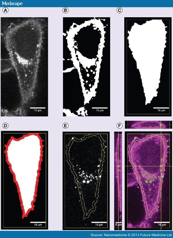
Figure 1.
Particle-in-cell-3D processing overview.
(A) Representative confocal cross-section image of a HeLa cell plasma membrane stained with CellMask™ Deep Red. (B) The image of (A) is transformed into a white mask. (C) Further segmentation processes form the final mask of the cell. (D) Afterwards, its outer border is shrunk to define the enlarged membrane region (in red) and the region inside the cell (in white). The procedure occurs throughout the image stack, leading to a 3D reconstruction of the system. (E) Membrane region outlines (in yellow) are employed to segment the image of the fluorescent particles. (F) Merged image with orthogonal views along the yellow lines displaying the entire stack. The cell plasma membrane appears in magenta, while the membrane region outlines are shown in yellow. Particles are assigned to two different regions: intracellular (in green) and the membrane region (in cyan).
In a subsequent step, the outer ROI is shrunk by a given distance set by the user (see 'Input of analysis parameters' section), generating the inner ROI. The distance between the inner and the outer ROIs defines the width (w) of the membrane region. This space can be used as a threshold between extracellular and intracellular volumes. Hence, particles bound to the apical membrane should appear in this region if an adequate value for w is set. The position and shape of the membrane region depends directly on the appearance of the apical plasma membrane. It means that experimental conditions, such as the choice of the membrane marker, labeling protocol and cell type might influence the final geometry of the membrane region. An easy and good procedure to stain the cell membrane is given in the 'Cell culture & incubation of cells with particles' section, while an example on how to estimate the extension of the membrane region is presented in the 'Cell segmentation strategy' section. The formation of a membrane region with an intracellular space by Particle-in-cell-3D is shown in Figure 1A–D.
The volume of the cell and of the subcellular regions are calculated in volumetric pixels (voxels) and then converted to µm3 according to the preset XY- and Z-scales.
Assignment of particles to different cellular regions Particles are classified and color-coded according to their position with respect to the inner and the outer ROIs (Figure 1E). In order to do so, the spatial coordinates describing the center of intensity of every single object are automatically measured and recorded by the ImageJ plugin 3D Object Counter.[104] Particle-in-cell-3D uses this information as input data. If the center of intensity of an object is located inside the inner ROI, it is assigned as intracellular and color-coded in green (the user can also set a different color). In addition, if it is positioned between the inner and the outer ROI, it is classified as belonging to the membrane region and color-coded in cyan (Figure 1F). It is important to note that only objects above the lower threshold for particles and within a preselected size range (in number of voxels) are analyzed (see the 'Routine 2: measurement of the fluorescence intensity of particles' section and 'Input of analysis parameters' section).
Finally, a text file is created containing a report documenting the input parameters and the results. In addition, the main processed images and results tables are saved.
Routine 2: Measurement of the Fluorescence Intensity of Particles All aspects of routine 1 are present in routine 2. Additionally, it is able to quantify the fluorescence intensity (IntDens; Equation 1) of all intracellular and membrane-associated objects.
Lower threshold & volume of particles The lower threshold applied to particles is a key parameter for correct quantification. Objects are selected for analysis based on this value, that is, only pixels with intensity values above the threshold enter the calculation. In addition, the user is given the possibility to set the minimum and maximum volume (number of voxels) of thresholded pixels to be considered as an object (see the 'Input of analysis parameters' section).
Total fluorescence intensity of particles in a region
The total IntDens (TIntDens) of a region (R) – intracellular or membrane region – is defined as the sum of the IntDens over all objects belonging to that region (Equation 2):

TIntDens is therefore proportional to the number of particles in the region where it is calculated and semiquantitative results can be achieved by comparing the TIntDens of different region or cells.
Routine 3: Counting the Absolute Number of Particles Routine 3 includes all features presented in routines 1 and 2. It additionally permits the absolute quantification of particle uptake on the single-cell level.
Particle number distribution in agglomerates The calculation is straightforward and the number of particles forming an object i is given by Equation 3:

The mean IntDens of a single particle can be measured via routine 4 (see the 'Routine 4: calibration to measure the mean intensity of single particles' section).
Absolute number of particles taken up by cells The total number of intracellular particles is calculated by simple addition over all particles within the inner ROI. The same consideration holds for the total number of membrane-associated particles, but this time accounting for all particles located within the inner and the outer ROIs. The general equation can be written as follows (Equation 4):

where i indexes all objects from 1 to n in the cellular region R.
Concentration of particles The concentration of particles within each region is obtained by dividing the number of particles by the respective cellular volume (Equation 5):

Concentration-based approaches can be useful for cases in which the volume ratio of the two regions differs over time or within cells. Since the volume, the concentration and the number of particles in each region are automatically saved in a report file, it is straightforward to calculate new parameters based on the particle concentration.
Routine 4: Calibration to Measure the Mean Intensity of Single Particles Routine 4 is used to obtain the distribution of IntDens of all objects. This parameter is essential for routines 3 and 5. From this data set one can derive the mean IntDens of a single particle. Objects of interest are automatically selected in the image of the particles and added to the ImageJ ROI Manager. One after the other, each selected object is measured. In the end, a report of results shows the IntDens of all evaluated objects. However, analyzed objects are not only comprised of single particles but also of agglomerates. It is necessary to exclude agglomerates from the data set to yield just the mean IntDens of individual particles. This can be verified by other means, for example, super-resolution microscopy. In this work we use STED microscopy to accomplish this task (see the 'Accuracy of absolute quantification' section).
Routine 5: Quantifying Particles in Cell-free Regions Routine 5 was designed to characterize the concentration and agglomeration of particles in control experiments without cells. This information is extremely relevant because the exposure of particles to cells in a monolayer culture may vary with time owing to sedimentation and diffusion of particles in the cell medium.[19] The user is requested to define the 3D ROI to be analyzed. Next, if the mean IntDens is known, the total number of particles, their concentration and the particle number distribution are calculated within the selected region as defined by Equations 3–5.
Input of analysis parameters The possibility of adapting the analysis parameters according to experimental conditions increases the flexibility of Particle-in-cell-3D. The following parameters have to be set by the user during analysis and are saved in a final report.
XY-scale This parameter is the image size of each pixel in real space. It corresponds to the magnification calibration of the microscope system. The XY-scale has to be entered in nm per pixel. This value, together with the Z-scale, is used to calculate the volume of the cell and the concentration of particles.
Z-scale or interslice distance The Z-scale is the depth of each volumetric pixel (voxel) in real space. It defines the distance between two adjacent images in an image stack. This parameter is directly given by the interslice distance that is set during acquisition in a confocal microscope. The units to be used are nm per pixel. To avoid under- and over-sampling, images should be acquired following the Nyquist criterion.[20]
Width of the cell membrane region This parameter defines the distance w in pixels between the inner and the outer ROIs. It is thereby equal to the width of the region between the intra- and the extra-cellular environments, which is the membrane region (Figure 1D). The membrane region represents a transition space every particle has to pass through to be internalized by a cell. One should keep in mind that the membrane region is typically much wider than the actual membrane. Another point to be considered is that the amount of membrane-associated particles depends on how cells are exposed to the particles and on how cells are treated prior to imaging. For example, particles that were loosely bound to the membrane may be removed during staining and washing steps.
Background to be subtracted This parameter is used to correct for the background present in the image stack of the particles. The entered value is subtracted from the intensity value of each pixel. If no subtraction is needed (e.g., background was removed by another method), this parameter should be set to 0.
Lower threshold for particles Only pixels with intensity values exceeding this threshold will be considered particles and thus analyzed. When a correct threshold is set, the bright spots associated with the fluorescent objects form clusters of adjacent pixels and only these pixels are evaluated. This choice is fundamental for the whole analysis process as it has major influence on the results. If the threshold is set too low, artifacts such as background noise and cellular autofluorescence might be counted as particles. On the other hand, if it is set too high, dimmer particles will not be considered and agglomerates will be overestimated. In summary, the threshold must be set as low as possible, but high enough to allow object segmentation. When absolute quantification is intended, the lower threshold should be the same as the one used during calibration.
Minimum & maximum number of voxels The volume of the objects under investigation (in number of voxels, after applying the lower threshold) can be used to eliminate background noise and to avoid analyzing dimmer or brighter objects. If absolute quantification is intended, these values should also be the same as the ones used during calibration.
Threshold for segmenting the cell This is the lower threshold value applied to segment the cell and define its position.
Mean IntDens of a single particle This value characterizes the mean fluorescence intensity of individual particles. It can be obtained from the data set provided by running routine 4. The mean IntDens is not necessary in routines 1 and 2, but crucial to calculate the absolute number of particles in routines 3 and 5.
Experimental Details
Preparation of Fluorescent Mesoporous Silica Nanoparticles PEGylated colloidal mesoporous silica NPs (CMS-NPs) of 50–80 nm in size (ellipsoids) were synthesized as described elsewhere.[21] CMS-NPs were functionalized at their periphery with aminopropyl- and PEG-groups through cocondensation, followed by grafting the cyanine dye Cy3 N-hydroxysuccinimide (NHS) ester. The dye labeling was carried out with an ethanolic suspension of the particles having a concentration of 1 mg/ml by adding 14.2 µl of dye Cy3 NHS ester solution (2 mg/ml in dimethylformamide). The reaction solution was stirred for 1 h at room temperature in the dark, then the Cy3-labeled CMS nanoparticles (CMS-NPs-Cy3) were collected by centrifugation (14000 rpm for 5 min), washed three-times with ethanol and finally redispersed in water to a final concentration of 0.5 mg/ml.
Preparation of Fluorescent Polystyrene Nanoparticles for STED & Confocal Microscopy Precision cover slips (LH24.1, Carl Roth GmbH) were cleaned with ethanol. 50 µl of poly-l-lysine 0.1% solution (Sigma-Aldrich) was applied onto each cover slip. After 5 min the solution was removed with a pipette and the cover slip left to dry in air. Commercially available fluorescent polystyrene beads with a diameter of 100 nm (Red FluoSpheres 100 nm, Invitrogen) were diluted 1:1000 in ethanol and sonicated for 10 min. 5 µl of this solution was then applied to the lysine-treated cover slips. After evaporation samples where mounted with 7 µl of 2,2'-thiodiethanol (Sigma Aldrich, diluted to 97% in phosphate buffered saline), put on an objective slide and sealed with nail varnish. Samples were imaged as described in the 'Super-resolution imaging of 100-nm nanoparticles' section.
Cell Culture & Incubation of Cells With Particles HeLa cells were grown in DMEM supplemented with 10% fetal calf serum (Invitrogen) in 5% CO2 humidified atmosphere at 37°C. Cells were seeded 24 or 48 h before imaging on collagen A Lab-Tek chamber slides (Thermo Fisher Scientific Inc.) in a density of 2.0 × 10⁴ or 1.0 × 10⁴ cells/cm2, respectively.
Cells were incubated with the CMS-NPs-Cy3 at a final concentration of 120–180 µg/ml. The particle solution was prepared in CO2-independent medium (Invitrogen) with 10% fetal calf serum, sonicated for 10 min and heated up to 37°C. Prior to live-cell imaging the membrane of the cells was stained with CellMask™ Deep Red (Invitrogen) by replacing the particle-containing cell medium by a staining solution. The latter was prepared by adding 0.2 µl of CellMask™ into 400 µl of cell medium. After 1–2 min of incubation, the staining solution was replaced by CO2-independent medium (Invitrogen) supplemented with 10% fetal calf serum.
Quenching Experiments The quenching experiments were carried out on a custom-built wide-field microscope based on the Nikon Eclipse Ti microscope, as described before.[22] Samples were Köhler illuminated through a Nikon Plan APO TIRF 60×/1.45 oil immersion objective with 532 nm laser light with an integration time of 300 ms, exciting Cy3. The fluorescence was separated from the excitation light and image sequences were captured with an electron multiplier charge-coupled device camera (iXon+, Andor Technology). Cy3 fluorescence was quenched by adding 10 µl of a 0.4% trypan blue solution into 400 µl medium in the observed chamber during image acquisition and gently mixed. As trypan blue is a cell membrane-impermeable dye it is not able to quench particles that have been taken up by the cells. By comparing images prior to and after quenching, the percentage of internalized particles is accessible. Quenching experiments were performed to validate Particle-in-cell-3D performance in segmenting the cell and in measuring the fraction of internalized particles (see the 'Cell segmentation strategy' section and the 'Fraction of particles internalized by single cells' section).
Spinning Disc Imaging for Uptake Experiments Uptake experiments with CMS-Cy3-NPs were performed on a spinning disc confocal fluorescence microscope based on Nikon Eclipse TE 2000-E equipped with a Nikon Apo TIRF 100×/1.49 oil immersion objective. Specimens were illuminated with laser light alternating between 488 and 633 nm, exciting Cy3 and the cell membrane stain, respectively. Image sequences were captured with an electron multiplier charge-coupled device camera (iXon DV887ECCS-BV, Andor Technology). Before being captured by the camera, the emission signal was split by a dichroic mirror at 592 nm. The bandpass detection filters used were 525/50 nm (Cy3 channel) and 730/140 nm (cell membrane stain channel). Exposure times were set to 300 ms. Z-stacks of single cells were imaged with an interslice distance of 166 nm, following the Nyquist criterion.[20]
Super-resolution Imaging of 100-nm Nanoparticles To evaluate the absolute quantification algorithm of Particle-in-cell-3D, samples were imaged with a custom-built STED microscope in confocal and super-resolution mode. The setup is based around a supercontinuum laser (SC-450-PP-HE, Fianium Ltd), which emits from 459 to 2000 nm at a repetition rate of 1 MHz.[23] In short, the laser light is split by a dichroic mirror (Z660 DCXR, AHF Analysentechnik AG). The short wavelength part is sent through an emission filter (z568/10×; AHF Analysentechnik AG) to provide the excitation band of 570 ± 5 nm. The long wavelength part is sent to a custom-built prism-based monochromator to yield the spectrum suitable for efficient depletion of the excited state in super-resolution mode (695–713 nm). For the purpose of spatial filtering the excitation and depletion beams are coupled into single-mode polarization maintaining fibers (PMC-630-4,2-NA010-3-APC-200-P for excitation and PMC-630-4,6-NA011-3-APC-150-P for STED beam, Schäfter & Kirchhoff GmbH). After collimation, the excitation beam is coupled into the optical path of a 1.4 NA oil objective (HCX PL APO 100×/1.40–0.70 oil CS, Leica Microsystems GmbH) by a dichroic mirror (585 DCXR, AHF Analysentechnik AG). The depletion beam first passes through a vortex phase plate (VPP-1b, RPC Photonics) to imprint the phase necessary to yield the Laguerre-Gaussian LG01 mode used in STED microscopy. Consecutively, the depletion beam is coupled into the axis of the objective by a dichroic mirror (Q690 SPXR, AHF Analysentechnik AG). Both beams pass through an achromatic λ/4 retarder (custom-made by Bernhard Halle Nachfl. GmbH) to yield perfect circular polarization for the depletion band. The sample is scanned by a high-speed piezo scanning stage setup (P-733.2DD for XY, P-753.11C for Z; both controlled by an E-712 controller with DDL feature enabled, Physik Instrumente GmbH & Co. KG). Fluorescence is collected by a single-photon counting module (SPCM-AQRH-13-FC, Perkin Elmer Inc.) after it has passed the two aforementioned dichroic mirrors and a detection filter (Brightline HC 629/56, AHF Analysentechnik AG). Control of the setup is provided by custom-written Labview software (Labview 2011, National Instruments Corp.).
The microscope can be operated in two modes, namely standard confocal and STED mode.[23] In the confocal mode, only the excitation beam is active while the depletion beam is inactivated by means of a mechanical shutter (04RDS501, CVI Melles Griot). Imaging in this mode yields diffraction-limited optical resolution (~λExcitation/[2NAObjective]). In STED mode, the excitation and STED beams are both focused onto the sample rendering a resolution well below its confocal counterpart (~40 nm in imaging plane XY as opposed to 250 nm in confocal mode).
In confocal mode stacks were recorded with an area of 30 × 30 µm, a pixel-size of 100 nm and an interslice distance of 220 nm using an excitation intensity <1 µW. After recording the confocal stack, the focus was set to the position of the confocal image yielding the maximum signal, the STED beam was turned on (STED beam intensity ~1 mW) and another image of the exact same area was recorded with a pixel size of 20 nm. Pixel dwell time was typically 280 µs in both modes. The time to switch from confocal to STED imaging mode was a couple of seconds (limited mainly by refocusing to the plane of interest).
Nanomedicine. 2013;8(11):1815-1828. © 2013 Future Medicine Ltd.