


1. Introduction
Particles subject to an acoustic field experience a net force, traditionally termed the acoustic radiation force, mostly due to pressure spatial inhomogeneities in the surrounding fluid. While the time average of the leading-order time-harmonic acoustic force vanishes, higher-order terms yield a mean net force on the particle. The application of this force has proven advantageous in various frameworks requiring the manipulation of small particles (of a size smaller than few millimetres) due to the tractable monitoring of the applied acoustic field. Consequently, acoustic radiation forces are used in a sequence of gas-particle applications, including the separation, sorting and filtering of particles by means of acoustic tweezers (Baudoin & Thomas Reference Baudoin and Thomas2020). This platform has emerged in recent years as a versatile and substance-unharmful tool for bioparticle manipulation across a broad range of particle sizes, from nano-scale exosomes to millimetric size bacteria (Ozcelik et al. Reference Ozcelik, Rufo, Guo, Gu, Li, Lata and Huang2018).
A large body of work concerns the study of the radiation force acting on particles subject to an acoustic field at continuum-flow conditions, as recently reviewed by Baudoin & Thomas (Reference Baudoin and Thomas2020). An early investigation has been carried out by King (Reference King1934), who derived an expression for the radiation force on a solid sphere in the inviscid (ideal flow) limit. Ever since, this theory has been extended to consider the effects of fluid viscosity (Doinikov Reference Doinikov1994; Danilov & Mironov Reference Danilov and Mironov2000; Annamalai, Balachandar & Parmar Reference Annamalai, Balachandar and Parmar2014), flow thermodynamic state (Doinikov Reference Doinikov1997; Karlsen & Bruus Reference Karlsen and Bruus2015), particle shape and type (Hasegawa & Yosioka Reference Hasegawa and Yosioka1969; Glynne-Jones et al. Reference Glynne-Jones, Mishra, Boltryk and Hill2013) and the waveform of impinging disturbance (Silva Reference Silva2011) on the acoustic force. Relying on the continuum description, these analyses become invalid for particle sizes  ${\lesssim }1\ \mathrm {\mu } \textrm {m}$ at standard atmospheric conditions, where the gas molecular mean-free path equals
  ${\approx }0.1\ \mathrm {\mu } \textrm {m}$ (Sone Reference Sone2007). Further smaller nano-sized particles should be treated at free-molecular (ballistic) conditions, where the effect of gas molecular collisions is negligible. To the best of our knowledge, this limit has not been investigated hitherto.
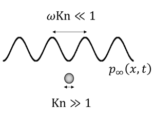
Noting the above, the objective of the present work is to analyse the acoustic radiation force on a rigid particle submerged in a gas at collisionless flow conditions. The investigation is carried out for a nano-sized sphere subject to a standing acoustic wave. The acoustic wavelength is assumed much larger than the sphere radius and molecular mean-free path, so that far-field continuum inviscid-flow conditions prevail. Different from existing finite-difference-based evaluations of the acoustic force about continuum-scale elements (Foresti, Nabavi & Poulikakos Reference Foresti, Nabavi and Poulikakos2012; Glynne-Jones et al. Reference Glynne-Jones, Mishra, Boltryk and Hill2013), counterpart non-continuum simulations (e.g. the direct simulation Monte Carlo method; see Bird Reference Bird1994) of nano-sized particles are presently impractical. This is due to the formidably costly computational resources necessary to resolve both small and large length scales of the particle and acoustic wavelength, respectively. In this context, the significance of the following analysis, yielding a closed-form evaluation for the free-molecular acoustic force, is evident.
2. Problem formulation and analysis
Consider a sphere of radius  $r_{0}^{*}$ (with asterisks hereafter denoting dimensional quantities) submerged in a nominally quiescent monatomic ideal gas of ambient density
  $\rho _0^*$ and temperature
  $T_{0}^{*}$. The sphere is subject to an acoustic field of wavelength
  $U_{{th}}^{*}/\omega ^{*}$, where
  $\omega ^{*}$ marks the wave frequency,
  $U_{{th}}^{*}=\sqrt {2\mathcal {R}^{*}T_{0}^{*}}$ denotes the most probable molecular speed and
  $\mathcal {R}^{*}$ is the specific gas constant. Taking
  $r_0^*$ and
  $U_{{th}}^{*}$ as the set-up normalizing length and velocity scales,
 \begin{equation} r=r^*/r_0^* \quad \mathrm{and}\quad u=u^*/U_{{th}}^{*}, \end{equation}
we construct the system Knudsen number and non-dimensional frequency,
 \begin{equation} {Kn}=\frac{l^{*}}{r_{0}^{*}}\quad \text{and}\quad \omega=\frac{\omega^{*}r_{0}^{*}}{U_{{th}}^{*}}, \end{equation}
respectively, where  $l^{*}$ denotes the gas molecular mean-free path. Focusing on a set-up where the acoustic wavelength is large compared with the molecular mean-free path, we obtain the non-dimensional restriction
  $\omega {Kn}\ll 1$. In accordance with gas kinetic theory, gases at low rarefaction rates (i.e. with small ratio of the molecular to the local macroscopic scale) are inviscid at leading order (Sone Reference Sone2007). Consequently, at large distances from the sphere (
 $r^*\gg r_0^*$), the effect of gas rarefaction becomes negligible and the flow field may be assumed ideal. In § 2.1 we describe the far acoustic field. The description obtained is then used in § 2.2 to derive an expression for the radiation force on the sphere.
2.1. Far acoustic field
We model the far acoustic field as a small-amplitude stationary acoustic wave oscillating along the  $x$-direction. Introducing the scaled acoustic pressure amplitude
 \begin{equation} \varepsilon=\frac{\varepsilon^{*}}{\rho_{0}^{*}U_{{th}}^{*2}}\ll1, \end{equation}
we expand
 \begin{equation} \varPhi=\varPhi^{(0)}+\varepsilon\varPhi^{(1)}(t,x)+\varepsilon^{2}\varPhi^{(2)}(t,x)+\cdots, \end{equation}
where  $\varPhi$ represents either the density
  $\rho$,
  $x$-velocity component
  $u$, pressure
  $p$ or temperature
  $T$. At leading order,
  $\rho ^{(0)}=T^{(0)}=1,u^{(0)}=0$ and
  $p^{(0)}=1/2$, in accordance with the scaled equation of state,
  $p=\rho T/2$. The
  $O(\varepsilon )$ continuum and inviscid
  $x$-momentum equations are supplemented by the isentropic relation,
  $p^{(1)}=c_{0}^{2}\rho ^{(1)}$, where
  $c_{0}=\sqrt {5/6}$ denotes the normalized speed of sound (in most probable speed units) for a monatomic gas. Solving the consequent
  $O(\varepsilon )$ one-dimensional wave equation for the pressure and placing the field antinode at
  $x=-h$, we obtain
 \begin{equation} \left.\begin{gathered} p^{(1)}(t,x)=\cos[\omega(x+h)/c_{0}]\cos(\omega t)\quad \text{and}\\ u^{(1)}(t,x)=\frac{1}{c_{0}}\sin[\omega(x+h)/c_{0}]\sin(\omega t). \end{gathered}\right\} \end{equation}
 Since the steady acoustic force is quadratic in  $\varepsilon$, the next-order correction in (2.4) should be calculated. To this end, the
  $O(\varepsilon ^{2})$ time-averaged inviscid
  $x$-momentum equation is given by
 \begin{equation} \frac{\partial\left\langle p^{(2)}\right\rangle }{\partial x}={-}\left\langle \rho^{(1)} \frac{\partial u^{(1)}}{\partial t}\right\rangle -\left\langle u^{(1)} \frac{\partial u^{(1)}}{\partial x}\right\rangle, \end{equation}
where  $\langle \cdot \rangle$ marks the time average over a period (
 $t_p=2{\rm \pi} /\omega$). Using the
  $O(\varepsilon )$
  $x$-momentum balance,
  $\partial u^{(1)}/\partial t=-\partial p^{(1)}/\partial x$, together with the isentropic
  $\rho ^{(1)}=6p^{(1)}/5$ relation, we obtain
 \begin{equation} \frac{\partial\left\langle p^{(2)}\right\rangle }{\partial x}= \frac{6}{5}\left\langle p^{(1)}\frac{\partial p^{(1)}}{\partial x}\right\rangle -\left\langle u^{(1)}\frac{\partial u^{(1)}}{\partial x}\right\rangle. \end{equation}
Integrating with  $x$, we find
 \begin{equation} \left\langle p^{(2)}\right\rangle =\tfrac{3}{5}\left\langle \left(p^{(1)}\right)^{2}\right\rangle -\tfrac{1}{2}\left\langle \left(u^{(1)}\right)^{2}\right\rangle, \end{equation}
indicating that the average pressure at second order equals the difference between the average acoustic potential energy and gas kinetic energy. Here, the constant of integration was eliminated as it does not contribute to the steady force on the particle. Applying a similar procedure to the  $O(\varepsilon ^{2})$ time-averaged continuity balance we obtain
 \begin{equation} \left\langle u^{(2)}\right\rangle ={-}\tfrac{6}{5}\left\langle p^{(1)}u^{(1)}\right\rangle =0, \end{equation}
where (2.5a,b) has been used to yield the vanishing of  $\langle p^{(1)}u^{(1)}\rangle$ and therefore of
  $\langle u^{(2)}\rangle$. The contribution of the constant of integration to
  $\langle u^{(2)}\rangle$, representing the system acoustic streaming, was eliminated from (2.9), as it results in a uniform-velocity-induced drag on the particle that is not in the focus of the present work.
Having determined  $\langle p^{(2)}\rangle$ and
  $\langle u^{(2)}\rangle$,
  $\langle \rho ^{(2)}\rangle$ and
  $\langle T^{(2)}\rangle$ may be obtained. Using the
  $O(\varepsilon ^{2})$ time-averaged equation of state for an ideal gas and applying (2.8), we find
 \begin{equation} \left\langle \rho^{(2)}\right\rangle +\left\langle T^{(2)}\right\rangle =2\left\langle p^{(2)}\right\rangle -\left\langle \rho^{(1)}T^{(1)}\right\rangle =\tfrac{6}{25}\left\langle \left(p^{(1)}\right)^{2}\right\rangle -\left\langle \left(u^{(1)}\right)^{2}\right\rangle. \end{equation}
Generally, the  $O(\varepsilon ^{2})$ energy balance should subsequently be imposed to yield an additional relation between
  $\langle \rho ^{(2)}\rangle$ and
  $\langle T^{(2)}\rangle$. Yet, the
  $O(\varepsilon ^{2})$ time-average inviscid energy equation is satisfied for any choice of
  $\langle \rho ^{(2)}\rangle$ and
  $\langle T^{(2)}\rangle$, implying that they can only be obtained by considering the viscous Navier–Stokes-Fourier transport equations at vanishingly small (yet non-zero)
  $\omega \mathrm {Kn}\ll 1$. Such a formulation would involve effects of gas heating due to viscous dissipation and would depend on the specific details of thermal boundary conditions on the far sound transducer and reflector surfaces. These effects are not treated here, yet the force due to an imposed far-field steady temperature gradient – namely, the thermophoretic force – has been considered in previous investigations (Sone Reference Sone2007). In the present work we wish to separate between the contributions of acoustic and thermophoretic forces, to allow for a comparison with existing continuum-limit results. For this purpose, we consider hereafter an adiabatic spherical particle. In this case, as shown in § 2.2 (see (2.22), (2.23) et seq.), the contributions of
  $\langle \rho ^{(2)}\rangle$ and
  $\langle T^{(2)}\rangle$ to the steady force form uniquely as their sum, evaluated in (2.10). Apart from separating between the acoustic and thermophoretic problems, the adiabatic condition renders the formulation simpler compared with the isothermal sphere set-up, thus enabling a more straightforward illustration of the effect of gas rarefaction on the calculated force. The omission of the viscous terms in (2.5a,b) and (2.6) neglects
  $O(\omega {Kn})\ll 1$ components in the acoustic field, resulting in a similar-order error in the evaluated radiation force for a long stationary wave.
2.2. Free-molecular near field
We consider a spherical particle of radius  $r_0^*$ much smaller than the molecular mean-free path
  $l^*$, so that
  ${Kn}\gg 1$. Combined with the previously prescribed condition of
  $\omega {Kn}\ll 1$ (see (2.2a,b) et seq.), this requires that
  $\omega \ll 1$. The effect of molecular collisions in the vicinity of the sphere is then negligible, and the near flow field is governed by the collisionless Boltzmann equation. This has been established in previous works on flow set-ups containing small-size objects (e.g. the thermophoretic motion of a sphere (Sone Reference Sone2007) and the generation of sound by actuated cylindrical (Ben Ami & Manela Reference Ben Ami and Manela2017) and spherical (Ben-Ami & Manela Reference Ben-Ami and Manela2019) bodies), showing the vanishing impact of the surface-reflected particles on the distribution function of the impinging gas molecules. Consequently, the gas adjacent to the sphere consists of: (i) molecules arriving from the far field with a probability density function
  $f_{\infty }(t,\boldsymbol {x},\boldsymbol {\xi })$ governed by the far inviscid conditions; (ii) molecules that diffusely reflect from the spherical surface with a probability density function
  $f_{w}(t,\boldsymbol {x},\boldsymbol {\xi })$. The inviscid conditions at infinity identify
  $f_{\infty }(t,\boldsymbol {x},\boldsymbol {\xi })$ as a local Maxwellian distribution (Sone Reference Sone2007). Expanding
  $f_{\infty }(t,\boldsymbol {x},\boldsymbol {\xi })$ in powers of
  $\varepsilon$ up to
  $O(\varepsilon ^2)$, we obtain
 \begin{align} f_{\infty}(t,\boldsymbol{x},\boldsymbol{\xi}) &\approx \frac{\mathrm{e}^{-\xi^{2}}}{{\rm \pi}^{3/2}}\left[1+\varepsilon\phi_{\infty}^{(1)}+ \varepsilon^{2}\left\langle \phi_{\infty}^{(2)}\right\rangle \right] =\frac{\mathrm{e}^{-\xi^{2}}}{{\rm \pi}^{3/2}}\left[1+\varepsilon\left(2\xi_{x}u^{(1)}+ \frac{4}{5}\xi^{2}p^{(1)}\right) \right.\nonumber\\ &\quad +\left.\varepsilon^{2}\left(\left\langle \rho^{(2)}\right\rangle + \left\langle T^{(2)}\right\rangle (\xi^{2}-3/2)+\left(2\xi_{x}^{2}-1\right) \left\langle \left(u^{(1)}\right)^{2}\right\rangle \right.\right.\nonumber\\ &\quad \left.\left.+\frac{2}{25}\left\langle \left(p^{(1)}\right)^{2}\right\rangle ({-}3-8\xi^{2}+4\xi^{4})\right)\right], \end{align}
where  $\xi \equiv |\boldsymbol {\xi }|$ is the magnitude of the molecular velocity vector
  $\boldsymbol {\xi }=(\xi _x,\xi _y,\xi _z)$ and time-harmonic components have been omitted from the
  $O(\varepsilon ^2)$ time-average term. Considering
  $f_{w}(t,\boldsymbol {x},\boldsymbol {\xi })$, the molecules reflected diffusely from the sphere acquire a Maxwellian distribution containing the spherical surface properties. A similar power expansion yields
 \begin{align} f_{w}(t,\boldsymbol{x},\boldsymbol{\xi})&\approx\frac{\mathrm{e}^{-\xi^{2}}}{{\rm \pi}^{3/2}} \left[1+\varepsilon\phi_{w}^{(1)}+\varepsilon^{2}\left\langle \phi_{w}^{(2)}\right\rangle \right] \nonumber\\ &=\frac{\mathrm{e}^{-\xi^{2}}}{{\rm \pi}^{3/2}} \left[1+\varepsilon\left(\rho_{w}^{(1)}+2\xi_{x}u_{p}^{(1)}+T_{w}^{(1)}(\xi^{2}-3/2)\right) \right.\nonumber\\ &\quad +\varepsilon^{2}\left(\left\langle \rho_{w}^{(2)}\right\rangle + \left(\left\langle T_{w}^{(2)}\right\rangle +\left\langle \rho_{w}^{(1)}T_{w}^{(1)}\right\rangle \right) \left(\xi^{2}-\frac{3}{2}\right)+\left(2\xi_{x}^{2}-1\right) \left\langle \left(u_{p}^{(1)}\right)^{2}\right\rangle\right.\nonumber\\ &\quad \left.\left. +\left\langle \left(T_{w}^{(1)}\right)^{2}\right\rangle \left(\frac{15}{8}-\frac{5}{2}\xi^{2}+\frac{1}{2}\xi^{4}\right)\right)\right], \end{align}
where  $u_{p}^{(1)}$ denotes the (a priori unknown) first-order particle velocity in the
  $x$-direction resulting from the applied acoustic field. The surface outgoing flux,
  $\rho _{w}^{(1),(2)}$, and temperature,
  $T_{w}^{(1),(2)}$, perturbations should be obtained through the imposition of impermeability and adiabatic wall conditions, described below.
2.2.1. First-order wall functions
Applying the impermeability condition at  $O(\varepsilon )$ at the spherical surface
  $r=1$, we obtain
 \begin{align} & \frac{1}{2{\rm \pi}^{3/2}} \int_{0}^{2{\rm \pi}}\mathrm{d}\varphi_{\xi} \int_{0}^{\infty}\xi^{3}\mathrm{e}^{-\xi^{2}}\mathrm{d}\xi \left[\int_{0}^{{\rm \pi}/2}\phi_{w}^{(1)}\sin(2\theta_{\xi})\mathrm{d}\theta_{\xi}+ \int_{{\rm \pi}/2}^{\rm \pi}\phi_{\infty}^{(1)}\sin(2\theta_{\xi}) \,\mathrm{d}\theta_{\xi}\right]_{r=1} \nonumber\\ &\quad =u_{p}^{(1)}\cos\theta, \end{align}
where the spherical-coordinate representation of  $\boldsymbol \xi =(\xi _r,\xi _\theta ,\xi _\varphi )$ is used,
  $\cos \theta _{\xi }=\xi _r / \xi$ and
  $\tan \varphi _{\xi }=\xi _{\theta } / \xi _{\varphi }$. Assuming an adiabatic sphere, the surface temperature is treated unknown and is determined through the application of a zero-heat-flux condition at
  $r=1$. At
  $O(\varepsilon )$ this yields
 \begin{equation} \int_{0}^{2{\rm \pi}}\mathrm{d}\varphi_{\xi}\int_{0}^{\infty}\xi^{5} \mathrm{e}^{-\xi^{2}}\mathrm{d}\xi\left[\int_{0}^{{\rm \pi}/2}\phi_{w}^{(1)}\sin(2\theta_{\xi})\mathrm{d} \theta_{\xi}+\int_{{\rm \pi}/2}^{\rm \pi}\phi_{\infty}^{(1)}\sin(2\theta_{\xi}) \,\mathrm{d}\theta_{\xi} \right]_{r=1}=0. \end{equation}
Integrating (2.13) and (2.14), we obtain
 \begin{equation} \left.\begin{gathered} \rho_{w}^{(1)}=\left[\frac{7\sqrt{\rm \pi}}{8}\left(u_{p}^{(1)}-u^{(1)}\right) \cos\theta+\frac{6}{5}p^{(1)}\right]_{r=1} \quad \mathrm{and}\\ {T}_{w}^{(1)}=\left[\frac{\sqrt{\rm \pi}}{4}\left(u_{p}^{(1)}-u^{(1)}\right)\cos\theta+ \frac{4}{5}p^{(1)}\right]_{r=1}, \end{gathered}\right\} \end{equation}
where  $u_{p}^{(1)}$ may be evaluated using Newton's second law,
 \begin{equation} \frac{4{\rm \pi}}{3}\rho_{p/g}\frac{\mathrm{d}u_{p}^{(1)}}{\mathrm{d}t}=F_{x}^{(1)}. \end{equation}
Here,  $\rho _{p/g}=\rho _{p}^{*}/\rho _{0}^{*}$ denotes the ratio of particle to gas densities, and
  $F_{x}^{(1)}$ marks the leading-order
  $x$-directed force on the sphere. Using scaling arguments, we find
 \begin{equation} u_{p}^{(1)}\sim\frac{F_{x}^{(1)}(\omega)}{\omega\rho_{p/g}}.\end{equation}
Implicit calculation of  $F_{x}^{(1)}$ (given in Appendix A) shows that
  $F_{x}^{(1)}(\omega )\sim \omega$ for
  $\omega \ll 1$. It is therefore established that, for the prevailing set-up of particles much heavier than the ambient gas (
 $\rho _{p/g}\gg 1$, common for solid particles),
  $u_{p}^{(1)}\ll u^{(1)}$ and
  $u_{p}^{(1)}$ may be neglected in (2.15a,b). The diminishing effect of particle oscillatory motion on the acoustic force for
  $\rho _{p/g}\gtrsim 10^2$ was similarly reported in Annamalai et al. (Reference Annamalai, Balachandar and Parmar2014) at continuum-flow conditions.
2.2.2. Second-order wall functions and steady acoustic force
Following a similar procedure to obtain  $\rho _w^{(2)}$ and
  $T_w^{(2)}$ in (2.12), we formulate the respective
  $O(\varepsilon ^2)$ time-averaged impermeability,
 \begin{equation} \int_{0}^{2{\rm \pi}}\mathrm{d}\varphi_{\xi}\int_{0}^{\infty}\xi^{3}\mathrm{e}^{-\xi^{2}} \mathrm{d}\xi\left[\int_{0}^{{\rm \pi}/2}\phi_{w}^{(2)}\sin(2\theta_{\xi})\,\mathrm{d}\theta_{\xi} +\int_{{\rm \pi}/2}^{\rm \pi}\phi_{\infty}^{(2)}\sin(2\theta_{\xi})\,\mathrm{d}\theta_{\xi}\right]_{r=1}=0, \end{equation}
and adiabatic,
 \begin{align} & -2\left\langle v_{\theta}^{(1)}\int_{0}^{2{\rm \pi}}\sin\varphi_{\xi}\mathrm{d}\varphi_{\xi} \int_{0}^{\infty}\xi^{4}\,\mathrm{e}^{-\xi^{2}}\,\mathrm{d}\xi\left[\int_{0}^{{\rm \pi}/2}\phi_{w}^{(1)} \sin^{2}\theta_{\xi}\cos\theta_{\xi}\,\mathrm{d}\theta_{\xi} \right.\right. \nonumber\\ &\quad \left.\left.\vphantom{\int_{0}^{{\rm \pi}/2}} +\int_{{\rm \pi}/2}^{\rm \pi}\phi_{\infty}^{(1)} \sin^{2}\theta_{\xi}\cos\theta_{\xi}\,\mathrm{d}\theta_{\xi}\right]\right\rangle_{r=1} \nonumber\\ &\quad +\frac{1}{2}\int_{0}^{2{\rm \pi}}\mathrm{d}\varphi_{\xi}\int_{0}^{\infty}\xi^{5}\, \mathrm{e}^{-\xi^{2}}\,\mathrm{d}\xi\left[\int_{0}^{{\rm \pi}/2}\left\langle \phi_{w}^{(2)}\right\rangle \sin(2\theta_{\xi})\,\mathrm{d}\theta_{\xi} \right. \nonumber\\ &\quad \left.\vphantom{\int_{0}^{{\rm \pi}/2}} +\int_{{\rm \pi}/2}^{\rm \pi}\left\langle \phi_{\infty}^{(2)}\right\rangle \sin(2\theta_{\xi})\mathrm{d}\theta_{\xi}\right]_{r=1}=0, \end{align}
wall conditions. In (2.19), the first-order tangential velocity  $v_{\theta }^{(1)}$ over the sphere surface is evaluated through
 \begin{align} v_{\theta}^{(1)}(r=1) &= \frac{1}{{\rm \pi}^{3/2}}\int_{0}^{2{\rm \pi}}\sin\varphi_{\xi}\mathrm{d}\varphi_{\xi} \int_{0}^{\infty}\xi^{3}\mathrm{e}^{-\xi^{2}}\mathrm{d}\xi\left[\int_{0}^{{\rm \pi}/2} \left\langle \phi_{w}^{(1)}\right\rangle \sin^{2}\theta_{\xi}\mathrm{d}\theta_{\xi}\right. \nonumber\\ &\quad \left.\vphantom{\int_{0}^{{\rm \pi}/2}} +\int_{{\rm \pi}/2}^{\rm \pi}\left\langle \phi_{\infty}^{(1)}\right\rangle \sin^{2} \theta_{\xi}\,\mathrm{d}\theta_{\xi}\right]_{r=1}={-}\frac{u^{(1)}(r=1)\sin\theta}{2}. \end{align}
Integrating (2.18) and (2.19) and assigning (2.10) yields
 \begin{equation} \left\langle \rho_{w}^{(2)}\right\rangle +\left\langle T_{w}^{(2)}\right\rangle = \frac{6}{25}\left\langle \left(p^{(1)}\right)^{2}_{r=1}\right\rangle -\left\langle \left(u^{(1)}\right)^{2}_{r=1}\right\rangle \left(1-\left(\frac{3}{2}-\frac{29{\rm \pi}}{128}\right) \cos^{2}\theta\right). \end{equation}
As shown below, and in similar to the discussion following (2.10), the steady acoustic force on the adiabatic sphere depends on the sum of  $\rho _{w}^{(2)}$ and
  $T_{w}^{(2)}$ only and not on their separate values, which are therefore not computed here.
Having analysed the  $O(\varepsilon ^2)$ wall functions, the general expression for the steady acoustic force on the sphere is given by
 \begin{equation} \left\langle F_{x}^{(2)}\right\rangle ={-}2{\rm \pi}\int_{0}^{\rm \pi} \left[\left\langle \sigma_{rr}^{(2)}(r=1)\right\rangle \cos\theta-\left\langle \sigma_{r\theta}^{(2)}(r=1) \right\rangle \sin\theta\right]\sin\theta\,\mathrm{d}\theta, \end{equation}
where  $\sigma _{rr}^{(2)}(r=1)$ and
  $\sigma _{r\theta }^{(2)}(r=1)$ denote the second-order normal and shear stresses along the sphere, respectively. Importantly, (2.22) assumes that the sphere displacement,
  $x_p$, is small compared to its radius (i.e.
  $x_p\ll 1$), so that a fixed reference surface surrounding the particle may be introduced and a ‘stationary’ force balance could be carried out. Focusing on a heavy (relative to the gas) sphere, it may be shown that
  $x_p\sim {\varepsilon }/{(\omega \rho _{p/g})}$ (see (2.17) et seq.). Indeed, this condition is satisfied over a wide range of parameters, where
  $\rho _{p/g}\gg 1$ and
  $\omega$ and
  $\varepsilon$ are similarly small, in line with the long-wavelength and linearization assumptions, respectively.
The time-averaged normal stress component appearing in (2.22) forms as
 \begin{align} \left\langle \sigma_{rr}^{(2)}(r=1)\right\rangle &= \frac{1}{{\rm \pi}^{3/2}}\int_{0}^{2{\rm \pi}}\mathrm{d}\varphi_{\xi} \int_0^{\infty}\xi^{4}\mathrm{e}^{-\xi^{2}}\,\mathrm{d}\xi \nonumber\\ &\quad \times\left[\int_{0}^{{\rm \pi}/2}\left\langle \phi_{w}^{(2)}\right\rangle \cos^{2}\theta_{\xi}\sin\theta_{\xi}\,\mathrm{d}\theta_{\xi}+\int_{{\rm \pi}/2}^{\rm \pi} \left\langle \phi_{\infty}^{(2)}\right\rangle \cos^{2} \theta_{\xi}\sin\theta_{\xi}\mathrm{d}\theta_{\xi}\right]_{r=1} \nonumber\\ &=\frac{1}{4}\left[\left\langle \rho_{w}^{(2)}\right\rangle +\left\langle T_{w}^{(2)}\right\rangle + \left\langle \rho_{w}^{(1)}T_{w}^{(1)}\right\rangle +\left\langle \rho^{(2)}\right\rangle +\left\langle T^{(2)}\right\rangle +\frac{24}{25}\left\langle \left(p^{(1)}\right)^{2}\right\rangle \right. \nonumber\\ &\quad \left.+2 \left\langle \left(u^{(1)}\right)^{2}\right\rangle \cos^{2}\theta\right]_{r=1}, \end{align}
indicating its specific dependence on  $\langle \rho ^{(2)}\rangle +\langle T^{(2)}\rangle$ and
  $\langle \rho _w^{(2)}\rangle +\langle T_w^{(2)}\rangle$ evaluated in (2.10) and (2.21), respectively. Using these relations,
  $\langle \sigma _{rr}^{(2)}(r=1)\rangle$ is expressed by
 \begin{equation} \left\langle \sigma_{rr}^{(2)}(r=1)\right\rangle = \left[\frac{3}{5} \left\langle \left(p^{(1)}\right)^{2}\right\rangle +\left\langle \left(u^{(1)}\right)^{2}\right\rangle \left(-\frac{1}{2} +\left(\frac{7}{8}-\frac{\rm \pi}{512}\right)\cos^{2}\theta\right)\right]_{r=1}. \end{equation}
The time-averaged second-order wall shear stress is given by
 \begin{align} \left\langle \sigma_{r\theta}^{(2)}(r=1)\right\rangle &={-}\frac{1}{2{\rm \pi}^{3/2}}\left\langle v_{\theta}^{(1)} \int_{0}^{2{\rm \pi}}\mathrm{d}\varphi_{\xi}\int_0^{\infty}\xi^{3}\,\mathrm{e}^{-\xi^{2}}\,\mathrm{d}\xi \left[\int_{0}^{{\rm \pi}/2}\phi_{w}^{(1)}\sin(2\theta_{\xi})\,\mathrm{d}\theta_{\xi} \right.\right. \nonumber\\ &\quad \left.\left.\vphantom{\int_{0}^{{\rm \pi}/2}} +\int_{{\rm \pi}/2}^{\rm \pi}\phi_{\infty}^{(1)}\sin(2\theta_{\xi})\,\mathrm{d}\theta_{\xi}\right]\right\rangle_{r=1} \nonumber\\ &\quad -\frac{1}{\sqrt{\rm \pi}}\left\langle \left(u^{(1)}\right)^{2}\right\rangle_{r=1} \sin(2\theta)\int_0^{\infty}\xi^{6}\,\mathrm{e}^{-\xi^{2}}\,\mathrm{d}\xi\int_{{\rm \pi}/2}^{\rm \pi} \cos^{2}\theta_{\xi}\sin^{3}\theta_{\xi}\,\mathrm{d}\theta_{\xi} \nonumber\\ &={-}\frac{1}{4}\sin(2\theta)\left\langle \left(u^{(1)}\right)^{2}\right\rangle_{r=1}, \end{align}
where (2.11), (2.12) and (2.20) have been applied.
To substitute (2.24) and (2.25) into (2.22) and carry out the required quadratures,  $p^{(1)}$ and
  $u^{(1)}$ in (2.5a,b) should be expressed in spherical coordinates. Towards this end, we expand
 \begin{align} & \left\langle \left(p^{(1)}\right)^{2}\right\rangle_{r=1} \nonumber\\ &\quad =\frac{\varPi^{2}}{8}\sum_{n=0}^{\infty}\sum_{m=0}^{\infty} \left\{(2n+1)(2m+1)\mathrm{i}{}^{n+m}j_{n}\left(\frac{\omega}{c_{0}}r\right)j_{m} \left(\frac{\omega}{c_{0}}r\right)P_{n}(\cos\theta)P_{m}(\cos\theta)\right. \nonumber\\ &\qquad \left.\times\left[({-}1)^{n}\exp\left(-\mathrm{i}\frac{\omega h}{c_{0}}\right)+ \exp\left(\mathrm{i}\frac{\omega h}{c_{0}}\right)\right]\left[({-}1)^{m} \exp\left(-\mathrm{i}\frac{\omega h}{c_{0}}\right)+ \exp\left(\mathrm{i}\frac{\omega h}{c_{0}}\right)\right]\right\} \end{align}
and
 \begin{align} & \left\langle \left(u^{(1)}\right)^{2}\right\rangle_{r=1} \nonumber\\ &\quad ={-}\frac{\varPi^{2}}{8c_0^2}\sum_{n=0}^{\infty}\sum_{m=0}^{\infty} \left\{(2n+1)(2m+1)\mathrm{i}{}^{n+m}j_{n}\left(\frac{\omega}{c_{0}}r\right)j_{m} \left(\frac{\omega}{c_{0}}r\right)P_{n}(\cos\theta)P_{m}(\cos\theta)\right. \nonumber\\ &\qquad \left.\times\left[({-}1)^{n}\exp\left(-\mathrm{i}\frac{\omega h}{c_{0}}\right)- \exp\left(\mathrm{i}\frac{\omega h}{c_{0}}\right)\right]\left[({-}1)^{m} \exp\left(-\mathrm{i}\frac{\omega h}{c_{0}}\right)- \exp\left(\mathrm{i}\frac{\omega h}{c_{0}}\right)\right]\right\}. \end{align}
Here,  $P_{n}$ denotes the Legendre polynomial of
  $n$th order and
  $j_n$ marks the
  $n$th-order spherical Bessel function of the first kind. Upon substitution of the expanded forms of
  $\langle (p^{(1)})^{2}\rangle _{r=1}$ and
  $\langle (u^{(1)})^{2}\rangle _{r=1}$ into (2.24) and (2.25) and then into (2.22), the orthogonality relations for triple products of the Legendre polynomials,
 \begin{equation} \left.\begin{gathered} \int_{0}^{\rm \pi}P_{1}(\cos\theta)P_{n}(\cos\theta)P_{n+1}(\cos\theta) \sin\theta\,\mathrm{d}\theta=\frac{(2n+2)}{(2n+1)(2n+3)} \quad \mathrm{and} \\ \int_{0}^{\rm \pi}P_{3}(\cos\theta)P_{n}(\cos\theta)P_{n+3}(\cos\theta)\sin\theta\,\mathrm{d}\theta= \frac{15}{24}\frac{(2n+2)(2n+4)(2n+6)}{(2n+1)(2n+3)(2n+5)(2n+7)}, \end{gathered}\right\}\end{equation}
are applied (Dougall Reference Dougall1953), yielding the desired expression for the free-molecular second-order steady acoustic force on the sphere,
 \begin{align} \left\langle F_{x}^{(2)}\right\rangle_{{fm}} &= \frac{3{\rm \pi}}{100}\sin\left(\frac{2\omega h}{c_0}\right)\sum_{n=0}^{\infty} \left[\left(11+\frac{3{\rm \pi}}{64}\right)({-}1)^{n}(2n+2)j_{n}\left(\frac{\omega}{c_0}\right)j_{n+1} \left(\frac{\omega}{c_0}\right)\right. \nonumber\\ &\quad \left.+\frac{5}{4}\left(3-\frac{\rm \pi}{64}\right)({-}1)^{n} \frac{(2n+2)(2n+4)(2n+6)}{(2n+3)(2n+5)}j_{n}\left(\frac{\omega}{c_0}\right)j_{n+3} \left(\frac{\omega}{c_0}\right)\right]. \end{align}
3. Discussion
As stated in the beginning of § 2.2, expression (2.29) for the steady acoustic force should be valid only for  $\omega \ll 1/{Kn}$, ensuring inviscid-flow conditions of the impinging acoustic wave. As additionally noted therein, since
  $\mathrm {Kn}\gg 1$, this implies that
  $\omega \ll 1$, and (2.29) may be simplified to yield the leading-order approximation
 \begin{equation} {\langle F_{x}^{(2)}\rangle_{{fm}}}\approx \frac{\rm \pi}{10c_0^2\sqrt{30}}\left(11+\frac{3{\rm \pi}}{64}\right) \sin\left(\frac{2\omega h}{c_0}\right)\omega+O(\omega^{3}) \quad \mathrm{as}\ \omega\ll1. \end{equation}
 To examine the feasibility of levitating the spherical particle through the applied acoustic field, we estimate the characteristic ratio between the amplitudes of the acoustic and gravitational forces operating on the sphere. Typically, for the free-molecular regime to be valid,  ${Kn}\gtrsim 10$, equivalent to a nano-sphere of radius
  $r_{0}^{*}\lesssim 10$ nm at atmospheric conditions. Additionally, to ensure far inviscid conditions, we require that
  $\omega {Kn}\lesssim 10^{-2}$, so that the standing-wave attenuation may be considered negligible (Ben Ami & Manela Reference Ben Ami and Manela2017). The above restrictions yield
  $\omega \lesssim 10^{-3}$, corresponding to a dimensional frequency of
  $\omega ^*\sim 1$ MHz for a nano-sized particle at atmospheric conditions with
  $U_{{th}}^*\approx 350$ m s
 $^{-1}$. Taking
  $\varepsilon \lesssim 10^{-1}$ to warrant linearized flow conditions (as supported by previous analyses of acoustic wave propagation in planar and non-planar geometries, e.g. Manela & Pogorelyuk Reference Manela and Pogorelyuk2015; Ben Ami & Manela Reference Ben Ami and Manela2017; Ben-Ami & Manela Reference Ben-Ami and Manela2019), we evaluate the acoustic to gravitational force ratio as
 \begin{equation} \frac{\varepsilon^2\langle F_{x}^{(2)}\rangle_{{fm}}}{F_g} \sim \frac{\varepsilon^2 U_{{th}}^{*2}\omega}{g^{*}r_{0}^{*}\rho_{p/g}} \lesssim10^{4},\end{equation}
where  $g^{*}\approx 10\ \mathrm {m}~\mathrm {s}^{-2}$ marks the dimensional gravitational acceleration and the particle to gas densities ratio was taken
  $\rho _{p/g}\approx 10^3$. Evidently, the large characteristic ratio obtained implies that the long-wavelength-induced acoustic field may be useful in levitating nano-particles.
Having demonstrated the above, it is of interest to compare the ballistic-limit result with former evaluations of the steady force in the continuum regime (where  ${Kn}\ll 1$) at large acoustic wavelengths (
 $\omega \ll 1$) (King Reference King1934; Doinikov Reference Doinikov1994). To this end, we start by rescaling expression (3.1) for the free-molecular force to read
 \begin{equation} Y_{{fm}}=\frac{\langle F_{x}^{(2)}\rangle_{{fm}}}{\dfrac{\rm \pi}{2c_0^2} \sin\left(\dfrac{2\omega h}{c_0}\right)}\approx \frac{1}{30}\sqrt{\frac{6}{5}}\left(11+\frac{3{\rm \pi}}{64}\right)\omega+O(\omega^{3}) \quad \mathrm{as}\ \omega\ll1, \end{equation}
reducing the harmonic dependence of  $\langle F_{x}^{(2)}\rangle _{{fm}}$ on the prescribed position
  $x=-h$ of the acoustic wave antinode. Next, consider (6.14) and (7.6) in Doinikov (Reference Doinikov1994) for the case of a standing acoustic wave impinging on a ‘fastened’ sphere (
 $\rho _{p/g}\gg 1$). We focus on the limits of a viscous layer much smaller or larger than the sphere radius. Applying the current scaling, these correspond to set-ups with
  ${Kn}\ll \omega$ and
  ${Kn}\gg \omega$, respectively, where we make use of the viscosity-based definition of the Knudsen number,
 \begin{equation} {Kn}={2\nu^{*}}/{(U_{{th}}^{*}r_{0}^{*})}. \end{equation}
Here,  $\nu ^{*}$ marks the gas mean kinematic viscosity, and the factor 2 is introduced such that
  $({Kn}/\omega )^{1/2}$ specifies the ratio between the viscous boundary-layer width and the sphere radius,
  $[2\nu ^{*}/(\omega ^{*}r_{0}^{*2})]^{1/2}$ (Doinikov Reference Doinikov1994). In (6.14) and (7.6) of Doinikov (Reference Doinikov1994), the amplitude of the wave velocity potential
  $A^{*}$ may be recast as
  $A^{*}=\varepsilon U_{{th}}^{*2}/\omega ^{*}$ to correspond to current notation. Scaling the force in Doinikov (Reference Doinikov1994) by
  ${{\rm \pi} \varepsilon ^2} r_{0}^{*2}\rho _{0}^{*}U_{{th}}^{*2}/{(2c_0^2)}$, the non-dimensional force in the continuum limit is given by
 \begin{equation} Y_{{cont}}\approx\begin{cases} \dfrac{5}{3}\sqrt{\dfrac{6}{5}}\omega\left(1+\dfrac{9}{10} \sqrt{\dfrac{{Kn}}{\omega}}\right), & {Kn}\ll\omega\ll1,\\ \dfrac{9}{5}\sqrt{\dfrac{6\omega{Kn}}{5}} \left(1+\dfrac{10}{27}\sqrt{\dfrac{\omega}{{Kn}}}\right), & \omega\ll {Kn}\ll1. \end{cases}\end{equation}
Notably, the result in (3.5) (as in other works concerning the problem in the continuum limit) does not consider the impact of fluid velocity slip over the spherical surface at non-zero  ${Kn}$. It is nevertheless reasonable to assume that this effect, typically proportional to
  ${Kn}\ll 1$ (Sone Reference Sone2007), should only slightly affect the acoustic force in the limit of small Knudsen numbers. The free-molecular and continuum-limit results are compared in figure 1. The blue solid curve presents the force obtained in (2.29) for
  ${Kn}\gg 1$ using
  $N=20$ terms of the series, whereas the dashed-blue line shows its
  $\omega \ll 1$ leading-order approximation given in (3.3). We observe that the two curves are nearly indiscernible for
  $\omega \lesssim 0.2$, implying that the leading-order approximation (3.3) is sufficient for capturing the force in the free-molecular limit. As discussed above (see (3.1) et seq.), free-molecular conditions are expected to hold at low frequencies that should not exceed
  $\omega \lesssim 0.2$.

Figure 1. Variation with  $\omega$ of the steady acoustic force on a sphere in the free-molecular (blue curves) and continuum (black lines) regimes. The solid blue curve corresponds to the force calculated in (2.29) (with 20 terms of the series), while the dashed blue line presents its
  $\omega \ll 1$ leading-order term given in (3.3). The dashed black lines mark the continuum-limit results obtained in Doinikov (Reference Doinikov1994) for
  ${Kn}=0.01$ (see (3.5)).
Inspecting the forces in the free-molecular and continuum limits, we notice that the latter are larger in the entire range of  $\omega \ll 1$ considered. In the case
  ${Kn}\ll \omega$ (where the viscous boundary layer is thin compared with the sphere radius),
  $Y_{{cont}}\propto \omega$, similarly to
  $Y_{{fm}}$ (cf. (3.3)). Yet, the magnitude of the continuum-limit force is approximately five times larger than its free-molecular counterpart. Physically, for
  ${Kn}\ll \omega$, the acoustic force in the continuum limit is dominated by the contribution of pressure distribution over the sphere, whereas the shear stress and the non-isotropic contributions to the deviatoric part of the normal stress are scaled with
  ${Kn}$. Conversely, these terms turn
  $O(1)$ at free-molecular conditions (see
  $\langle \sigma _{r\theta }^{(2)}\rangle$ in (2.25) and the
  $\cos ^{2}\theta$ term of
  $\langle \sigma _{rr}^{(2)}\rangle$ in (2.24)), counteract the pressure contribution and diminish the total force. Using kinetic-level arguments, while the effect of molecular collisions at continuum-limit conditions leads to transformation of far-field
  $x$-momentum into excess pressure on the sphere, the absence of collisions in the free-molecular limit results in partial ‘escape’ of wall-reflected momentum to the far field. Traversing to the
  $\omega \ll {Kn}$ regime, the dominant contribution to the continuum-limit force is due to the viscous-shear component. Here, the non-dimensional force is proportional to the width of the viscous boundary layer scaled by the acoustic wavelength,
  $\sim \sqrt {\omega {Kn}}$. This results in a slower decrease as
  $\omega \rightarrow 0$ relative to the
  $\sim \omega$ reduction in the free-molecular limit, where a viscous layer cannot be defined.
4. Conclusions
We studied the steady acoustic force, imposed by a long-wavelength standing acoustic wave in an ideal gas, on a sphere of radius much smaller than the molecular mean-free path. A closed-form expression was obtained for the steady force on an adiabatic nano-sphere (for which  ${Kn}\gg 1$) submerged in a long-wavelength field (where
  $\omega {Kn}\ll 1$). While the force on an otherwise isothermal particle was not considered in the present work, it may be readily obtained by subsequently solving for the
  $O(\varepsilon ^{2})$ far-field steady temperature deviation in the gas, which depends on specific modelling of the far sound generator and reflector surfaces. Comparison between the current free-molecular and previous continuum-limit (Doinikov Reference Doinikov1994) analyses of the acoustic force at long-wavelength (
 $\omega \ll 1$) conditions revealed a typical five times larger force in the latter case at a given non-dimensional frequency. This was rationalized in terms of momentum ‘escape’ at free-molecular conditions by molecules reflected from the solid particle. Inspecting the amplitude of the free-molecular force, we found that it may become up to four orders of magnitude larger than the gravitational force, thus suggesting the viability of applying an acoustic field for the manipulation of nano-scale particles.
While the current work constructs a theoretical framework for the calculation of free-molecular acoustic forces on small-scale particles, it is yet desirable to examine the breakdown of the scheme with decreasing  ${Kn}$. This may be carried out by either employing non-continuum simulations (e.g. the direct simulation Monte Carlo method; Bird Reference Bird1994) or by directly solving the kinetic Boltzmann equation. However, such analyses appear particularly challenging, mainly due to the formidable computational effort required to capture both small and large length scales of the particle and sound wave, respectively. One approach for overcoming this difficulty may be the application of a hybrid simulation method (e.g. the scheme presented by Stephani, Goldstein & Varghese Reference Stephani, Goldstein and Varghese2013), where the far acoustic field, calculated via continuum equations, is matched with a kinetic-simulation computation in the vicinity of the particle. This approach may allow the calculation of the long-wavelength acoustic force on particles in the entire range of Knudsen numbers, and its application constitutes a topic for a future investigation.
Funding
The research was supported by the Israel Science Foundation (grant no. 1084/16) and the Aeronautical Engineering Research Fund. Y.B. acknowledges the support by the Adams Fellowship Program of the Israel Academy of Sciences and Humanities.
Declaration of interests
The authors report no conflict of interest.
Appendix A. Evaluation of  $F_x^{(1)}$

The expression for  $F_x^{(1)}$ forms similarly to (2.22) for
  $\langle F_x^{(2)}\rangle$, after removing the time-average operator and replacing the second-order with a first-order notation. This yields
 \begin{equation} {F}_{x}^{(1)}={-}2{\rm \pi}\int_{0}^{\rm \pi}\left[{\sigma}_{rr}^{(1)}(r=1)\cos\theta-{\sigma}_{r\theta}^{(1)}(r=1) \sin\theta\right]\sin\theta\,\mathrm{d}\theta, \end{equation}
where  $r$ and
  $\theta$ mark the radial coordinate and azimuthal angle relative to the
  $x$-direction in spherical coordinates, respectively. The
  $O(\varepsilon )$ normal and shear stresses along the sphere in (A1) are given by
 \begin{align} \sigma_{rr}^{(1)}\left(r=1\right) &= \frac{2}{\sqrt{\rm \pi}}\left[\int_{0}^{\infty}\xi^{4} \,\textrm{e}^{-\xi^{2}}\mathrm{d}\xi\int_{0}^{{\rm \pi}/2}\phi_{w}^{(1)}\cos^{2}\theta_{\xi} \sin\theta_{\xi}\mathrm{d}\theta_{\xi}\right. \nonumber\\ &\quad +\left.\vphantom{\int_{0}^{{\rm \pi}/2}} \int_{0}^{\infty}\xi^{4}\,\textrm{e}^{-\xi^{2}}\,\mathrm{d}\xi \int_{{\rm \pi}/2}^{\rm \pi}\phi_{\infty}^{(1)}\cos^{2}\theta_{\xi} \sin\theta_{\xi}\,\mathrm{d}\theta_{\xi}\right]_{r=1} \nonumber\\ &= p^{(1)}\left(r=1\right)-\cos\theta\left(\frac{9\sqrt{\rm \pi}}{32}+ \frac{1}{\sqrt{\rm \pi}}\right)u^{(1)}\left(r=1\right) \end{align}
and
 \begin{align} \sigma_{r\theta}^{(1)}\left(r=1\right) &={-}\frac{2 u^{(1)}\left(r=1\right)\sin\theta}{\sqrt{\rm \pi}} \int_{0}^{\infty}\xi^{5}\,\textrm{e}^{-\xi^{2}}\,\mathrm{d}\xi \nonumber\\ &\quad \times\int_{{\rm \pi}/2}^{\rm \pi}\cos\theta_{\xi}\sin^{3}\theta_{\xi}\,\mathrm{d}\theta_{\xi} =\frac{u^{(1)}\left(r=1\right)}{2\sqrt{\rm \pi}}\sin\theta, \end{align}
respectively. Transferring  $p^{(1)}$ and
  $u^{(1)}$ to the frequency domain,
 \begin{equation} \left\{ p,u\right\} ^{(1)}(t,x)=\tfrac{1}{2}\left[\left\{ \bar{p},\bar{u}\right\}^{(1)}(x) \exp\left[\mathrm{i}\omega t\right]+\mathrm{c.c.}\right] \end{equation}
(with  $\mathrm {c.c.}$ denoting the complex conjugate of a complex function), and expanding
  $\{ \bar {p},\bar {u}\} ^{(1)}$ in spherical coordinates, we write
 \begin{equation} \bar{p}^{(1)}=\frac{1}{2}\sum_{n=0}^{\infty}(2n+1)\mathrm{i}{}^{n}j_{n} \left(\frac{\omega}{c_{0}}r\right)P_{n}(\cos\theta)\left[({-}1)^{n} \exp\left(-\mathrm{i}\frac{\omega h}{c_{0}}\right)+ \exp\left(\mathrm{i}\frac{\omega h}{c_{0}}\right)\right] \end{equation}
and
 \begin{equation} \bar{u}^{(1)}=\frac{1}{2c_{0}}\sum_{n=0}^{\infty}(2n+1)\mathrm{i}{}^{n}j_{n} \left(\frac{\omega}{c_{0}}r\right)P_{n}(\cos\theta)\left[({-}1)^{n} \exp\left(-\mathrm{i}\frac{\omega h}{c_{0}}\right)- \exp\left(\mathrm{i}\frac{\omega h}{c_{0}}\right)\right], \end{equation}
where we have applied the identity (Arfken & Weber Reference Arfken and Weber2005)
 \begin{equation} \exp\left(\mathrm{i}\frac{\omega}{c_{0}}x\right)=\exp\left(\mathrm{i} \frac{\omega}{c_{0}}r\cos\theta\right)=\sum_{n=0}^{\infty}(2n+1)\mathrm{i}{}^{n}j_{n} \left(\frac{\omega}{c_{0}}r\right)P_{n}(\cos\theta) \end{equation}
and used the notations  $j_{n}$ and
  $P_{n}$ for the
  $n$th-order spherical Bessel function and Legendre polynomial, respectively. Substituting (A5) and (A6) into (A2) and (A3), we obtain
 \begin{align} \bar{\sigma}_{rr}^{(1)}\left(r=1\right) &= \frac{1}{2}\sum_{n=0}^{\infty}(2n+1)\mathrm{i}{}^{n}j_{n} \left(\frac{\omega}{c_{0}}\right)P_{n}(\cos\theta) \nonumber\\ &\quad \times\left\{ \left[({-}1)^{n}\exp\left(-\mathrm{i}\frac{\omega}{c_{0}}h\right)+ \exp\left(\mathrm{i}\frac{\omega}{c_{0}}h\right)\right]\right. \nonumber\\ &\quad \left.-\frac{1}{c_{0}}\left(\frac{9\sqrt{\rm \pi}}{32}+\frac{1}{\sqrt{\rm \pi}}\right) \cos\theta\left[({-}1)^{n}\exp\left(-\mathrm{i}\frac{\omega h}{c_{0}}\right)- \exp\left(\mathrm{i}\frac{\omega h}{c_{0}}\right)\right]\right\} \end{align}
and
 \begin{align} \bar{\sigma}_{r\theta}^{(1)}\left(r=1\right) &= \frac{1}{2c_{0}\sqrt{\rm \pi}}\sin\theta\sum_{n=0}^{\infty}(2n+1)\mathrm{i}{}^{n}j_{n}\left(\frac{\omega} {c_{0}}\right)P_{n}(\cos\theta) \nonumber\\ &\quad \times\left[({-}1)^{n}\exp\left(-\mathrm{i}\frac{\omega}{c_{0}}h\right)- \exp\left(\mathrm{i}\frac{\omega}{c_{0}}h\right)\right]. \end{align}
The expression for  $\bar {F}_{x}^{(1)}$ is then
 \begin{align} \bar{F}_{x}^{(1)} &={-}2{\rm \pi}\int_{0}^{\rm \pi}\left(\bar{\sigma}_{rr}^{(1)}(r=1) \cos\theta-\bar{\sigma}_{r\theta}^{(1)}(r=1)\sin\theta\right)\sin\theta\,\mathrm{d}\theta \nonumber\\ &={-}\frac{4{\rm \pi}}{c_{0}}\sin\left(\frac{\omega}{c_{0}}h\right)\left[\mathrm{i} \left(\frac{3\sqrt{\rm \pi}}{32}+\frac{1}{\sqrt{\rm \pi}}\right)j_{0} \left(\frac{\omega}{c_{0}}\right)-c_{0}j_{1}\left(\frac{\omega}{c_{0}}\right)- \frac{3\mathrm{i}}{16}\sqrt{\rm \pi}j_{2}\left(\frac{\omega}{c_{0}}\right)\right], \end{align}
and  ${F}_{x}^{(1)}$ follows from application of the operator in (A4) to (A10).


 Open access